Predicting Object Bounding Boxes and Road Map Layouts in a Traffic Environment

Summary

In today’s everchanging technological eras, one of the most exciting and hotly-debated advancements is that of self-driving cars. While the realization of such a futuristic piece of technology requires the coordination of many talents, from engineers to software developers to computer vision experts, the fundamental first step, as with any problem, is how best to represent the world around you. In this paper, we apply a pre-processing step of stitching together six 360 degree images into a single representation, then apply the YOLOv3 architecture for the task of object detection of nearby cars, trucks, and other vehicles. Our architecture transforms this into the two-dimensional road map representation, wherein additional autonomous decision-making would be applied to determine what best action the vehicle should take. For the road map prediction task, our model develops an average representation methodology based on labeled road images from the given dataset.

Report can be found here, slides here and relevant code can be found in this GitHub repo.

Data and Methods

The data used for this project consists of labeled and unlabeled scenes taken from a moving car. The data is organized into three levels: scene, sample, and image. A scene comprises 25 seconds of a car’s journey. Within each scene, a sample is a snapshot of the scene occurring at every 0.2 seconds. Each sample contains six images, taken with cameras pointing 60 degrees apart in order to create a complete 360 degree sample of what is going around the car. Each scene contains 126 samples, each with 6 images. The unlabeled dataset consists of 106 scenes while the labeled dataset contains 28 scenes, indicating a semi-supervised analysis. Additionally, there is extra information present for each sample, describing the current state of the car (stopped, lane change, turn, etc), that can be used to further enhance the model with particular specifications.

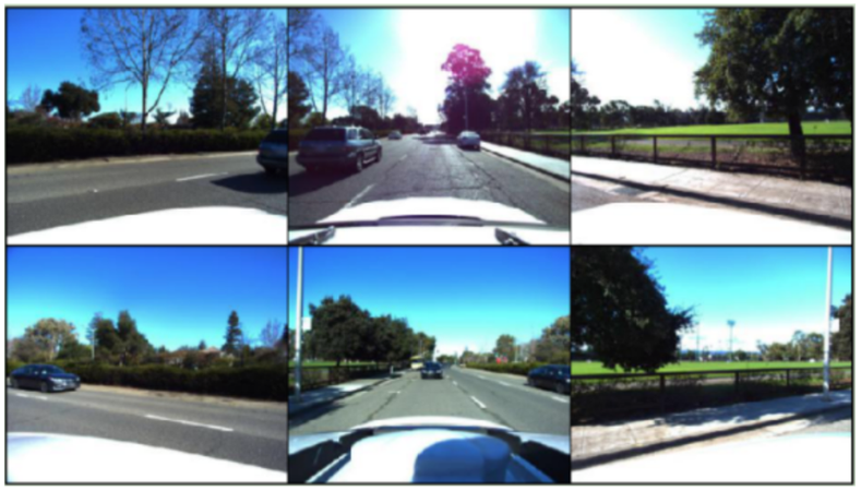
We considered different representations, including passing each image separately, a flat left-to-right (256x306*6) stitching, and flipping the back three images upside-down and placing them underneath the front three images. However, these representations were not the correct way to represent the image we were concerned with outputting. We believed that if our inputs could as closely as possible resemble a two-dimensional top-down representation, that would work the best in predicting the bounding boxes. To accomplish this, the sides were combined in the following order right (front back), forward behind, and left (front back). The front images are assembled on the left and the back images on the right. The front images are all rotated 90 degrees counterclockwise while the back images are all rotated 90 degrees clockwise.

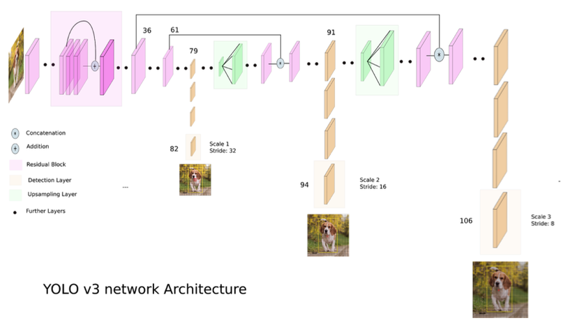
We used the YOLOv3 architecture for the bounding box task. It uses a variant of Darknet-53 as its feature extractor and comprises a total of 106 convolutional layers. The object detection is performed at three different scales. For our purposes, these three scales were determined by down-sampling the dimensions of the input image by 32, 16 and 8. Finally, it takes the generated bounding boxes and applies non-maximum suppression to group boxes together. As discussed earlier, the images were stitched together to get the objects as close to their position in a top-down view as possible. The annotations were also transformed to the format expected by the model, i.e. for each box, we passed the coordinates of the center of the box (assuming the bottom left corner to be the origin) and the width and height of the box. We also passed the specific object category to our labels so that our model could learn to identify the type of object in addition to being able to better determine the size of the corresponding bounding box. Currently our model can only draw boxes parallel to the axes and this can be explored as a next step.

Given the imbalance of data between labeled and unlabeled scenes (28 to 106), there will be an added benefit of using the stitched representations of the input images. Despite this, the overall reliability of these stitched images in terms of two-dimensional top-down roads is not very representative of the output we are aimed at predicting. For this reason, our model considers only the labeled road images. This allowed us to experiment with different techniques and we ended up returning the average road layout of the entire labeled dataset. This value was thresholded at 0.5 in order to create a binary road layout.

For both tasks, threat score (ts) is the chosen evaluation metric. In the binary road map task, the model is evaluated on average threat score (ts) as defined below:

Evaluating on the test set, our model obtained threat scores of 0.001 on the bounding box task and 0.68 on the road map task. For the bounding box, the model is evaluated across a range of thresholds (0.5, 0.6, 0.7, 0.8, 0.9). The metric is calculated as the weighted average over the union of the five thresholds. Models perform better given more time to train.