Least Squares GAN Image Generation

Summary

Generative Adversarial Networks (GAN) have been proven successful in generating images which seem realistic. However, typical GAN’s utilize a sigmoid loss function, which can often lead to mode collapse and the failure of the model to produce authentic images. In this paper, we reproduce the successes of previous work demonstrating that using a least squares loss function will lead to improved stability in generating realistic images. We evaluate the success of this improved model by training over the Fashion-MNIST dataset.

Report can be found here, poster here and relevant code can be found in this GitHub repo.

Data and Methods

We used the PyTorch package to implement both our GAN and LSGAN, and trained both over the Fashion-MNIST dataset, a set of 60,000 images of shoes, shirts, dresses, pants, and other articles of clothing. In addition to the sigmoid vs least squares loss function for GAN vs LSGAN, we also experimented with architectures of various complexities, as well as batch normalization. We used GPU’s configured on Google Colab to train each model for 200 epochs, then manually examined the resulting images produced, assessing them for image quality, blurriness, and how much they resemble actual articles of clothing. Additionally, for each model we calculated the Frechet Inception Distance (FID), a metric evaluating the similarity between generated images and the real images they were trained on.

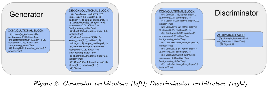
To implement these models, we adapted architectures from the LSGAN paper as closely as possible, making minor simplifications in reducing the number of layers in order to decrease run-time and prevent mode collapse, discussed further below. The architecture of our GAN’s and LSGAN’s are nearly identical, with the main difference being the choice of sigmoid vs least squares loss function. The loss functions of the LSGAN is slightly more complex because of the square loss, as shown below:

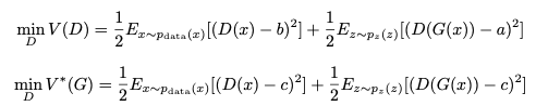
There are several combinations to choosing a,b, and c, one being if b − c = 1 and b − a = 2, then the LSGAN minimizes the Pearson χ2 Divergence between $2p_{g}(x)$ and $pdata(x) + p_{g}(x)$. We used parameters a = 0, b = c = 1. This choice of parameters does not minimize the divergence, but it still enables the generator to generate realistic images, and has similar performance.

In terms of both quality of images generated and FID score, we observed that the LSGAN without batch normalization performed best. We observed that overall, the GAN was more likely to exhibit “mode collapse”, wherein the generator is unable to improve itself. In fact, in many runs it would generate blurry images which didn’t look like articles of clothing whatsoever. When this happened, the generator loss typically began increasing without ever improving, and the discriminator loss converges to zero, meaning the model is failing to produce images which could be mistaken as true images. To remedy this, we tried decreasing the complexity of our model by reducing the number of convolutional and deconvolutional layers, particularly in the discriminator. This yielded better results, though the LSGAN still performed best overall.